Loan default prediction
In this tutorial you will use the getML Python API in order to
The main result is the analysis of a real world problem from the financial sector. You will learn how to tackle a data science problem from scratch to a production-ready solution.
Introduction
This tutorial features a use case from the financial sector. We will use getML in order to predict loan default. A loan is the lending of money to companies or individuals. Banks grant loans in exchange for the promise of repayment. Loan default is defined as the failure to meet this legal obligation, for example when a home buyer fails to make a mortgage payment. It is essential for a bank to estimate the risk it carries when granting loans to potentially non-performing customers.
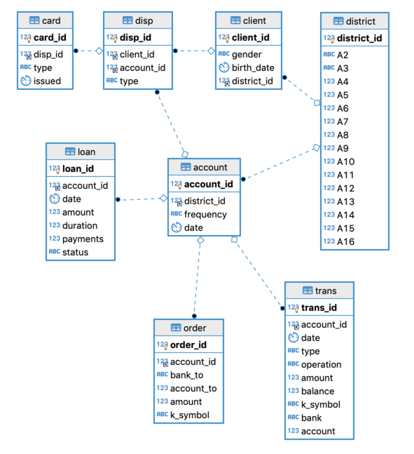
The analysis is based on the financial dataset from the the CTU Prague Relational Learning Repository. It contains information about 606 successful and 76 not successful loans and consists of 8 tables:
The loan table contains information about the loans granted by the
bank, such as the date of creation, the amount, and the planned duration
of the loan. It also contains the status of the loan. This is the
target variable that we will predict in this analysis. The loan
table is connected to the table account via the column
account_id.
The account table contains further information about the accounts
associated with each loan. Static characteristics such as the date of
creation are given in account and dynamic characteristics such as
debited payments and balances are given in order and trans. The
table client contains characteristics of the account owners. Clients
and accounts are related via the table disp. The card table
describes credit card services the bank offers to its clients and is
related to a certain account also via the table disp. The table
district contains publicly available information such as the
unemployment rate about the districts a certain account or client is
related to. More information about the dataset can be found
here.
In the following, we will further explore the data and prepare a data model to be used for the analysis with getML. As usual, we start with setting a project.
import getml
getml.engine.set_project('loans')
Creating new project 'loans'
Since the data sets from the CTU Prague Relational Learning Repository are available from a MariaDB database, we use getML’s data base connector to directly load the data into the getML engine.
getml.database.connect_mysql(
    host="relational.fit.cvut.cz",
    port=3306,
    dbname="financial",
    user="guest",
    password="relational",
    time_formats=['%Y/%m/%d']
)

loan = getml.data.DataFrame.from_db('loan', name='loan')
account = getml.data.DataFrame.from_db('account', name='account')
order = getml.data.DataFrame.from_db('order', name='order')
trans = getml.data.DataFrame.from_db('trans', name='trans')
card = getml.data.DataFrame.from_db('card', name='card')
client = getml.data.DataFrame.from_db('client', name='client')
disp = getml.data.DataFrame.from_db('disp', name='disp')
district = getml.data.DataFrame.from_db('district', name='district')
Data preparation
We will have a closer look at the tables from the financial dataset and setup the data model. Note that a convenient way to explore the data frames we just loaded into the getML engine is to have a look at them in the getML monitor. We recommend to check what is going on there in parallel to this tutorial.
Setting roles
In order to tell getML feature engineering algorithms how to treat the columns of each Data Frame we need to set its role. For more info in roles check out the user guide. The loan table looks like this
| loan_id | account_id | amount | duration | date | payments | status | |
|---|---|---|---|---|---|---|---|
| 0 | 4959.0 | 2.0 | 80952.0 | 24.0 | 1994-01-05 | 3373.00 | A |
| 1 | 4961.0 | 19.0 | 30276.0 | 12.0 | 1996-04-29 | 2523.00 | B |
| 2 | 4962.0 | 25.0 | 30276.0 | 12.0 | 1997-12-08 | 2523.00 | A |
| 3 | 4967.0 | 37.0 | 318480.0 | 60.0 | 1998-10-14 | 5308.00 | D |
| 4 | 4968.0 | 38.0 | 110736.0 | 48.0 | 1998-04-19 | 2307.00 | C |
| ... | ... | ... | ... | ... | ... | ... | ... |
| 677 | 7294.0 | 11327.0 | 39168.0 | 24.0 | 1998-09-27 | 1632.00 | C |
| 678 | 7295.0 | 11328.0 | 280440.0 | 60.0 | 1998-07-18 | 4674.00 | C |
| 679 | 7304.0 | 11349.0 | 419880.0 | 60.0 | 1995-10-29 | 6998.00 | C |
| 680 | 7305.0 | 11359.0 | 54024.0 | 12.0 | 1996-08-06 | 4502.00 | A |
| 681 | 7308.0 | 11362.0 | 129408.0 | 24.0 | 1996-12-27 | 5392.00 | A |
The status column is our target variable. It contains 4 different
categories:
A stands for contract finished, no problems,
B stands for contract finished, loan not paid,
C stands for running contract, OK so far,
D stands for running contract, client in debt
Before assigning it the role target we need to transform it to a
numerical variable. We will consider A and C a successfull loan and B
and D a default.
default = ((loan['status'] == 'B') | (loan['status'] == 'D'))
loan.add(default, name='default', role='target')
print(loan['default'].sum())
SUM aggregation, value: 76.0.
The data set contains 76 defaulted loans out of 681 data points in total, which corresponds to roughly 10%.
Next, ow we assign roles to the remaining columns in loan
join_key: loan_id, account_id
time_stamp: date
numerical: amount, duration, payments
Note that the column status, which obviously contains a data leak,
will not be considered by getML since we do not assign it a role.
loan.set_role(["account_id", "loan_id"], getml.data.roles.join_key)
loan.set_role(["date"], getml.data.roles.time_stamp)
loan.set_role(["amount", "duration", "payments"], getml.data.roles.numerical)
The account table looks like this
| account_id | district_id | frequency | date | |
|---|---|---|---|---|
| 0 | 1.0 | 18.0 | POPLATEK MESICNE | 1995-03-24 |
| 1 | 2.0 | 1.0 | POPLATEK MESICNE | 1993-02-26 |
| 2 | 3.0 | 5.0 | POPLATEK MESICNE | 1997-07-07 |
| 3 | 4.0 | 12.0 | POPLATEK MESICNE | 1996-02-21 |
| 4 | 5.0 | 15.0 | POPLATEK MESICNE | 1997-05-30 |
| ... | ... | ... | ... | ... |
| 4495 | 11333.0 | 8.0 | POPLATEK MESICNE | 1994-05-26 |
| 4496 | 11349.0 | 1.0 | POPLATEK TYDNE | 1995-05-26 |
| 4497 | 11359.0 | 61.0 | POPLATEK MESICNE | 1994-10-01 |
| 4498 | 11362.0 | 67.0 | POPLATEK MESICNE | 1995-10-14 |
| 4499 | 11382.0 | 74.0 | POPLATEK MESICNE | 1995-08-20 |
print(account['frequency'].count_distinct())
COUNT_DISTINCT aggregation, value: 3.0.
Frequency is a categorial variable with 3 distinct categories, so we add
it to the data model. Accordingly, we set the time_stamp and
join_key columns for account.
account.set_role(["account_id", "district_id"], getml.data.roles.join_key)
account.set_role(["date"], getml.data.roles.time_stamp)
account.set_role(["frequency"], getml.data.roles.categorical)
Population table
Let’s have a closer look at the relation between loans and
account:
print(loan['account_id'].count_distinct())
print(account['account_id'].count_distinct())
COUNT_DISTINCT aggregation, value: 682.0.
COUNT_DISTINCT aggregation, value: 4500.0.
The join key account_id has no duplicated value neither in loan
nor in account. That means, each row in loan is associated with
exactly one row in account. This is called a one-to-one relation.
It does not make sense to let getML’s feature engieering algorithms try to find aggregations over the accounts associated with each loan (because there is only one). So we perform the join operation between both tables before feeding to getML. This is part of the definition of the data model and is generally recommended for one-to-one or many-to-one relations. The resulting table will be the population table of our analysis.
population = loan.join(
    name='population',
    other=account,
    how='left',
    join_key='account_id',
    other_cols=[
        account['district_id'],
        account['frequency'],
        account['date'].alias('date_account')
    ]
)
| frequency | account_id | loan_id | district_id | amount | duration | payments | default | date | date_account | status | |
|---|---|---|---|---|---|---|---|---|---|---|---|
| 0 | POPLATEK MESICNE | 2 | 4959 | 1 | 80952.0 | 24.0 | 3373.0 | 0.0 | 1994-01-05 | 1993-02-26 | A |
| 1 | POPLATEK MESICNE | 19 | 4961 | 21 | 30276.0 | 12.0 | 2523.0 | 1.0 | 1996-04-29 | 1995-04-07 | B |
| 2 | POPLATEK MESICNE | 25 | 4962 | 68 | 30276.0 | 12.0 | 2523.0 | 0.0 | 1997-12-08 | 1996-07-28 | A |
| 3 | POPLATEK MESICNE | 37 | 4967 | 20 | 318480.0 | 60.0 | 5308.0 | 1.0 | 1998-10-14 | 1997-08-18 | D |
| 4 | POPLATEK TYDNE | 38 | 4968 | 19 | 110736.0 | 48.0 | 2307.0 | 0.0 | 1998-04-19 | 1997-08-08 | C |
| 5 | POPLATEK MESICNE | 67 | 4973 | 16 | 165960.0 | 24.0 | 6915.0 | 0.0 | 1996-05-02 | 1994-10-19 | A |
| 6 | POPLATEK MESICNE | 97 | 4986 | 74 | 102876.0 | 12.0 | 8573.0 | 0.0 | 1997-08-10 | 1996-05-05 | A |
| 7 | POPLATEK MESICNE | 103 | 4988 | 44 | 265320.0 | 36.0 | 7370.0 | 1.0 | 1997-12-06 | 1996-03-10 | D |
| 8 | POPLATEK MESICNE | 105 | 4989 | 21 | 352704.0 | 48.0 | 7348.0 | 0.0 | 1998-12-05 | 1997-07-10 | C |
| 9 | POPLATEK MESICNE | 110 | 4990 | 36 | 162576.0 | 36.0 | 4516.0 | 0.0 | 1997-09-08 | 1996-07-17 | C |
| ... | ... | ... | ... | ... | ... | ... | ... | ... | ... | ... | ... |
| 672 | POPLATEK MESICNE | 11231 | 7277 | 1 | 89280.0 | 12.0 | 7440.0 | 0.0 | 1997-10-24 | 1997-02-05 | A |
| 673 | POPLATEK MESICNE | 11244 | 7279 | 33 | 155760.0 | 24.0 | 6490.0 | 0.0 | 1997-12-11 | 1997-01-12 | C |
| 674 | POPLATEK MESICNE | 11265 | 7284 | 15 | 52788.0 | 12.0 | 4399.0 | 0.0 | 1993-09-15 | 1993-01-14 | A |
| 675 | POPLATEK MESICNE | 11271 | 7286 | 5 | 67320.0 | 36.0 | 1870.0 | 0.0 | 1997-01-31 | 1995-09-20 | C |
| 676 | POPLATEK MESICNE | 11317 | 7292 | 50 | 317460.0 | 60.0 | 5291.0 | 0.0 | 1998-11-22 | 1997-07-11 | C |
| 677 | POPLATEK MESICNE | 11327 | 7294 | 7 | 39168.0 | 24.0 | 1632.0 | 0.0 | 1998-09-27 | 1997-10-15 | C |
| 678 | POPLATEK MESICNE | 11328 | 7295 | 54 | 280440.0 | 60.0 | 4674.0 | 0.0 | 1998-07-18 | 1996-11-05 | C |
| 679 | POPLATEK TYDNE | 11349 | 7304 | 1 | 419880.0 | 60.0 | 6998.0 | 0.0 | 1995-10-29 | 1995-05-26 | C |
| 680 | POPLATEK MESICNE | 11359 | 7305 | 61 | 54024.0 | 12.0 | 4502.0 | 0.0 | 1996-08-06 | 1994-10-01 | A |
| 681 | POPLATEK MESICNE | 11362 | 7308 | 67 | 129408.0 | 24.0 | 5392.0 | 0.0 | 1996-12-27 | 1995-10-14 | A |
We also randomly split the data into a training and a validation set. We use 70% of the data set for training and the rest for testing.
split = 0.7
population_train = population.where('population_train', population.random() < split)
population_test = population.where('population_test', population.random() >= split)
Peripheral tables
The next step is to check the join relations between the population
table and the remaining peripheral tables. We start by considering
order and trans since the are both joined via account_id and
do not have any further relationships with other tables. We check if any
of the rows in population has a one-to-many relationship with
order (or trans). If it is the case, we cannot perform the join
relation directly but pass the peripheral table to getML’s feature
engieering algorithms in order to let them find the right aggregation
operations to create the best features.
import numpy as np

account_ids = population['account_id'].to_numpy()

for peri_ in [order, trans]:
    print(peri_.name)
    unique, counts = np.unique(peri_['account_id'].to_numpy(), return_counts=True)
    for acc_ in account_ids:
        idx = np.where(unique == float(acc_))[0]
        if counts[idx] > 1:
            print("-> has one-to-many")
            break
order
-> has one-to-many
trans
-> has one-to-many
Consequently we keep both order and trans as part of our
relational data model. Therefore we assign the columns in both tables
appropriate roles. Before assigning a column the role categorical we
make sure that the number of distinct categories is not too large.
print('order')
order.set_role(["account_id"], getml.data.roles.join_key)
order.set_role(["amount"], getml.data.roles.numerical)

for col_ in ["bank_to", "k_symbol", "account_to"]:
    unique_cat = len(np.unique(order[col_].to_numpy()))
    print("Distinct categories in {}: {}".format(col_, unique_cat))
    if unique_cat <= 20:
        order.set_role([col_], getml.data.roles.categorical)

print('trans')
trans.set_role(["account_id", "trans_id"], getml.data.roles.join_key)
trans.set_role(["date"], getml.data.roles.time_stamp)
trans.set_role(["amount", "balance"], getml.data.roles.numerical)

for col_ in ["type", "k_symbol", "bank","operation", "account"]:
    unique_cat = len(np.unique(trans[col_].to_numpy()))
    print("Distinct categories in {}: {}".format(col_, unique_cat))
    if unique_cat <= 20:
        trans.set_role([col_], getml.data.roles.categorical)
order
Distinct categories in bank_to: 13
Distinct categories in k_symbol: 5
Distinct categories in account_to: 6446
trans
Distinct categories in type: 3
Distinct categories in k_symbol: 9
Distinct categories in bank: 14
Distinct categories in operation: 6
Distinct categories in account: 768596
Setting units
Let’s stop here with adding peripheral tables to our data model and see
how far we can get with only the two tables trans and order.
There is, however, one more thing we can do: We can also to tell the
engine about the unit for each column. Columns will the same unit will
be compared in the feature engineering process. For more info check out
the user
guide.
loan.set_unit(["amount"], 'money')
order.set_unit(["amount"], 'money')
trans.set_unit(["amount", "balance"], 'money')
Data model
Now, we can formally define the data model. This is done using Placeholders. We can create these placeholder directly from the DataFrames.
population_placeholder = population.to_placeholder()
order_placeholder = order.to_placeholder()
trans_placeholder = trans.to_placeholder()
These Placeholders are then joined together in order to define the data model we will then turn over to the engine.
population_placeholder.join(order_placeholder,
                            join_key="account_id")
population_placeholder.join(trans_placeholder,
                            join_key="account_id",
                            time_stamp="date")
The final data model looks like this
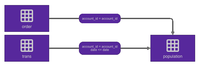
Training a Multirel Model
After having prepared the dataset we can dive into the actual analysis.
This is the point where getML sets in with automated feature engineering
and model training. We will train a MultirelModel in order to predict
the target column default. We will start with the default settings
and take care of the hyperparameter optimization later on. Input to the
model are a feature selector and a predictor. We will use XGBoost for
both in this tutorial.
feature_selector = getml.predictors.XGBoostClassifier(
    reg_lambda=500
)

predictor = getml.predictors.XGBoostClassifier(
    reg_lambda=500
)
We also need to provied the placeholders defined above. Now we are ready to instantiate the MultirelModel.
agg_ = getml.models.aggregations

model = getml.models.MultirelModel(
    aggregation=[
        agg_.Avg,
        agg_.Count,
        agg_.Max,
        agg_.Median,
        agg_.Min,
        agg_.Sum,
        agg_.Var
    ],
    num_features=30,
    population=population_placeholder,
    peripheral=[order_placeholder, trans_placeholder],
    loss_function=getml.models.loss_functions.CrossEntropyLoss(),
    feature_selector=feature_selector,
    predictor=predictor,
    seed=1706
).send()
The next step is to fit the model using the training data set.
model = model.fit(
    population_table=population_train,
    peripheral_tables=[order, trans]
)
Loaded data. Features are now being trained...
Trained model.
Time taken: 0h:0m:31.185045
The training time of the model is below one minute. Let’s look at how well the model performs on the validation dataset.
in_sample = model.score(
        population_table=population_train,
        peripheral_tables=[order, trans]
)

out_of_sample = model.score(
        population_table=population_test,
        peripheral_tables=[order, trans]
)
print("In sample accuracy: {:.2f}\nIn sample AUC: {:.2f}\nOut of sample accuracy: {:.2f}\nOut of sample AUC: {:.2f}".format(
    in_sample['accuracy'][0], in_sample['auc'][0], out_of_sample['accuracy'][0], out_of_sample['auc'][0]))
In sample accuracy: 0.94
In sample AUC: 0.92
Out of sample accuracy: 0.94
Out of sample AUC: 0.83
This is already a promising result but we can try to do better by performing a hyperparameter optimization.
Hyperparameter optimization
We will perform a hyperparamter optimization to improve the out of sample accuracy. We will do this using a Latin Hypercube search.
param_space = dict(
    grid_factor = [1.0, 16.0],
    max_length = [1, 10],
    num_features = [10, 100],
    regularization = [0.0, 0.01],
    share_aggregations = [0.01, 0.3],
    share_selected_features = [0.1, 1.0],
    shrinkage = [0.01, 0.4],
    predictor_n_estimators = [100, 400],
    predictor_max_depth = [3, 15],
    predictor_reg_lambda = [0.0, 1000.0]
)

latin_search = getml.hyperopt.LatinHypercubeSearch(
    model=model,
    param_space=param_space,
    # n_iter=30,
    # Set n_iter to a smaller value in order to make the notebook finish quickly
    n_iter=2,
    seed=1706
)

latin_search.fit(
  population_table_training=population_train,
  population_table_validation=population_test,
  peripheral_tables=[order, trans],
)
Launched hyperparameter optimization...
scores = latin_search.get_scores()
best_model_name = max(scores, key=lambda key: scores[key]['auc'])
print("Out of sample accuracy: {:.2f}".format(scores[best_model_name]['accuracy'][0]))
print("AUC: {:.2f}".format(scores[best_model_name]['auc'][0]))
Out of sample accuracy: 0.94
AUC: 0.93
The hyperparameter optimization has improved the in sample accuracy and AUC. These results will get even better when performing a more thorough hyperparameter optimization.
Extracting Features
So far, we have trained a MultirelModel and conducted a hyperparameter
optimization. But what did actually happened behind the scenes? In order
to gain insight into the features the Multirel Model has construced, we
will look at the in SQL code of the constructed features. This
information is available in the getML monitor or by caling to_sql on
a getML model. The feature with the highest importance looks like this.
This is a typical example for a feature generated by Multirel. You can
see the logic behind the aggregation, but its also clear that it would
have been impossible to come up with the specific values by hand or
using brute force approaches:
CREATE TABLE FEATURE_2 AS
SELECT MEDIAN( t1.date_account - t2.date ) AS feature_2,
       t1.account_id,
       t1.date
FROM (
     SELECT *,
            ROW_NUMBER() OVER ( ORDER BY account_id, date ASC ) AS rownum
     FROM population
) t1
LEFT JOIN trans t2
ON t1.account_id = t2.account_id
WHERE (
   ( t2.balance > 390.000000 AND t2.balance > 159331.000000 AND t1.date - t2.date <= 28.142857 )
OR ( t2.balance > 390.000000 AND t2.balance <= 159331.000000 AND t1.amount > 464288.000000 )
OR ( t2.balance <= 390.000000 AND t1.date_account - t2.date <= -148.000000 )
) AND t2.date <= t1.date
GROUP BY t1.rownum,
         t1.account_id,
         t1.date;
Results
We are able to predict loan default in the example dataset with an accuracy of over 95% and a very good AUC. With this result getML is in the top 1% of published solutions on this problem. The training time for the initial model was less than one minute. Together with the data preparation this project can easily be completed within one day.
You can use this tutorial as starting point for your own analysis or head over the other tutorials and the user guide if you want to learn more about the functionalty getML offers. Please contact us with your feedback about this tutorial or general inquiries. We also offer proof-of-concept project if you need help getting started with getML.