Get started with getML
In this example, you will learn about the basic concepts of getML. You will tackle a simple problem using the Python API in order to gain a technical understanding of the benefits of getML. More specifically, you will learn how to do the following:
You have not installed getML on your machine yet? Head over to the installation instructions before you get started.
Introduction
Automated machine learning (AutoML) has attracted a great deal of attention in recent years. The goal is to simplify the application of traditional machine learning methods to real world business problems by automating key steps of a data science project, such as feature extraction, model selection, and hyperparameter optimization. With AutoML, data scientists are able to develop and compare dozens of models, gain insights, generate predictions, and solve more business problems in less time.
While it is often claimed that AutoML covers the complete workflow of a data science project - from the raw data set to the deployable machine learning models - current solutions have one major drawback: They cannot handle real world business data. This data typically comes in the form relational data. The relevant information is scattered over a multitude of tables that are related via so-called join keys. In order to start an AutoML pipeline, a flat feature table has to be created from the raw relational data by hand. This step is called feature engineering and is a tedious and error-prone process that accounts for up to 90% of the time in a data science project.
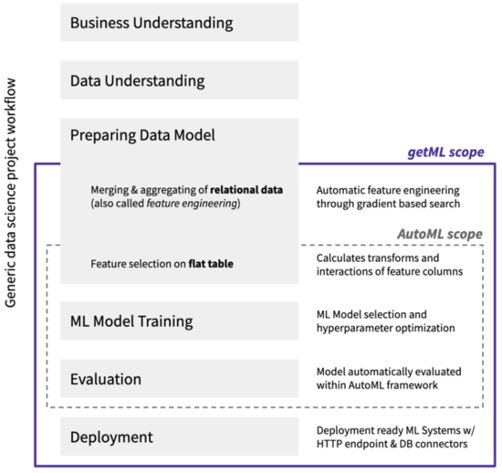
getML adds automated feature engineering on relational data and time series to AutoML. The getML algorithms, Multirel and Relboost, find the right aggregations and subconditions needed to construct meaningful features from the raw relational data. This is done by performing a sophisticated, gradient-boosting-based heuristic. In doing so, getML brings the vision of end-to-end automation of machine learning within reach for the first time. Note that getML also includes automated model deployment via a HTTP endpoint or database connectors. This topic is covered in other material.
All functionality of getML is implemented in the so-called getML engine. It is written in C++ to achieve the highest performance and efficiency possible and is responsible for all the heavy lifting. The getML Python API acts as a bridge to communicate with engine. In addition, the getML monitor provides a Go-based graphical user interface to ease working with getML and significantly accelerate your workflow.
In this article you will learn the basic steps and commands to tackle your data science projects using the Python API. For illustration purpose we will also touch how an example data set like the one used here would have been dealt with using classical data science tools. In contrast, we will show how the most tedious part of a data science project - merging and aggregating a relation data set - is automated using getML. At the end of this tutorial you are ready to tackle your own use cases with getML or dive deeper into our software using a variety of follow-up material.
Starting a new project
After you’ve successfully
installed
getML, you can launch it by executing the getml-cli command line
interface or double-clicking the application icon. This launches both
the getML engine and monitor.
Before diving into the actual project, you need to log into the getML suite. This happens in the getML Monitor, the frontend to the engine. If you open the browser of your choice and visit http://localhost:1709/, you’ll see a login screen. Click ‘create new account’ and follow the indicated steps. After you’ve activated your account by clicking the link in the activation E-mail you’re ready to go. From now on, the entire analysis is run from Python. We will cover the getML monitor in a later tutorial but feel free to check what is going on while following this guide.
import getml
print("getML version: {}".format(getml.__version__))
getML version: 0.10.0
First, we create a new project. All data sets and models belonging to a
project will be stored in ~/.getML/getml-VERSION/projects.
getml.engine.set_project('getting_started')
Creating new project 'getting_started'
Data set
The data set used in this tutorial consists of 2 tables. The so-called population table represents the entities we want to make a prediction about in the analysis. The peripheral table contains additional information and is related to the population table via a join key. Such a data set could appear for example in a customer churn analysis where each row in the population table represents a customer and each row in the peripheral table represents a transaction. It could also be part of a predictive maintenance campaign where each row in the population table corresponds to a particular machine in a production line and each row in the peripheral table to a measurement from a certain sensor.
In this guide, however, we do not assume any particular use case. After all, getML is applicable to a wide range of problems from different domains. Use cases from specific fields are covered in other articles.
population_table, peripheral_table = getml.datasets.make_numerical(
    n_rows_population=500,
    n_rows_peripheral=100000,
    random_state=1709
)

# Save data frames to disk in order to make them available after restarting the engine
population_table.save()
peripheral_table.save()
| time_stamp                  | join_key | column_01  |
| time stamp                  | join key | numerical  |
-------------------------------------------------------
| 1970-01-01T07:49:02.153328Z | 26       | -0.296267  |
| 1970-01-01T18:13:22.004830Z | 12       | 0.592168   |
| 1970-01-01T08:40:46.879346Z | 42       | -0.985272  |
| 1970-01-01T04:33:29.892692Z | 295      | 0.226407   |
| 1970-01-01T13:06:06.752214Z | 321      | -0.443054  |
| 1970-01-01T07:37:57.732301Z | 331      | 0.0363713  |
| 1970-01-01T11:35:47.812913Z | 380      | 0.62733    |
| 1970-01-01T23:48:30.471848Z | 39       | 0.253938   |
| 1970-01-01T00:56:13.548162Z | 389      | -0.952225  |
| 1970-01-01T05:57:45.546270Z | 281      | -0.0976082 |
| 1970-01-01T23:35:07.574544Z | 441      | 0.646095   |
| 1970-01-01T19:52:44.068679Z | 234      | 0.498297   |
| 1970-01-01T17:52:16.018061Z | 18       | 0.793115   |
| 1970-01-01T23:38:14.311144Z | 311      | -0.569989  |
| 1970-01-01T13:43:58.381644Z | 38       | 0.449462   |
| 1970-01-01T19:08:36.495451Z | 14       | 0.658454   |
| 1970-01-01T05:53:34.881204Z | 145      | 0.915759   |
| 1970-01-01T07:04:48.361633Z | 81       | 0.0773839  |
| 1970-01-01T16:08:21.021346Z | 195      | 0.513853   |
| 1970-01-01T11:15:32.595628Z | 304      | 0.115787   |
| ...                         | ...      | ...        |
This is the resulting population table
| join_key | column_01 | targets | time_stamp | |
|---|---|---|---|---|
| 0 | 0 | -0.629518 | 101.0 | 1970-01-01 11:18:00.114278400 |
| 1 | 1 | -0.962169 | 88.0 | 1970-01-01 21:35:41.185276800 |
| 2 | 2 | 0.732649 | 17.0 | 1970-01-01 02:03:27.430905600 |
| 3 | 3 | -0.462678 | 74.0 | 1970-01-01 08:45:55.322755200 |
| 4 | 4 | -0.837399 | 96.0 | 1970-01-01 10:37:51.538800000 |
| 5 | 5 | 0.322344 | 12.0 | 1970-01-01 01:36:50.690822400 |
| 6 | 6 | -0.670031 | 99.0 | 1970-01-01 13:33:29.236262400 |
| 7 | 7 | 0.551990 | 58.0 | 1970-01-01 06:13:30.637027200 |
| 8 | 8 | -0.793331 | 86.0 | 1970-01-01 23:44:02.882140800 |
| 9 | 9 | -0.009788 | 93.0 | 1970-01-01 17:43:11.392406400 |
| ... | ... | ... | ... | ... |
| 490 | 490 | -0.732420 | 97.0 | 1970-01-01 14:23:57.163315200 |
| 491 | 491 | 0.447224 | 55.0 | 1970-01-01 06:03:54.739900800 |
| 492 | 492 | -0.481879 | 62.0 | 1970-01-01 07:47:52.262966400 |
| 493 | 493 | -0.044106 | 99.0 | 1970-01-01 18:41:12.605395200 |
| 494 | 494 | -0.989142 | 87.0 | 1970-01-01 20:09:18.645177600 |
| 495 | 495 | 0.499767 | 93.0 | 1970-01-01 22:41:12.925276800 |
| 496 | 496 | -0.465699 | 101.0 | 1970-01-01 12:26:03.898233600 |
| 497 | 497 | 0.993191 | 59.0 | 1970-01-01 07:30:32.219683199 |
| 498 | 498 | 0.119690 | 92.0 | 1970-01-01 23:22:20.291030400 |
| 499 | 499 | -0.127432 | 101.0 | 1970-01-01 16:31:42.817382400 |
The population table contains 4 columns. The column called column_01
contains a random numerical value. The next column, targets, is the
one we want to predict in the analysis. To this end, we also need to use
the information from the peripheral table.
The relationship between the population and peripheral table is
established using the join_key and time_stamp columns: Join keys
are used to connect one or more rows from one table with one or more
rows from the other table. Time stamps are used to limit these joins by
enforcing causality and thus ensuring that no data from the future is
used during the training.
The peripheral table looks like this
| join_key | column_01 | time_stamp | |
|---|---|---|---|
| 0 | 26 | -0.296267 | 1970-01-01 07:49:02.153308800 |
| 1 | 12 | 0.592168 | 1970-01-01 18:13:22.004803200 |
| 2 | 42 | -0.985272 | 1970-01-01 08:40:46.879334400 |
| 3 | 295 | 0.226407 | 1970-01-01 04:33:29.892729599 |
| 4 | 321 | -0.443054 | 1970-01-01 13:06:06.752217600 |
| 5 | 331 | 0.036371 | 1970-01-01 07:37:57.732297600 |
| 6 | 380 | 0.627330 | 1970-01-01 11:35:47.812905600 |
| 7 | 39 | 0.253938 | 1970-01-01 23:48:30.471840000 |
| 8 | 389 | -0.952225 | 1970-01-01 00:56:13.548134400 |
| 9 | 281 | -0.097608 | 1970-01-01 05:57:45.546307200 |
| ... | ... | ... | ... |
| 99990 | 362 | 0.435637 | 1970-01-01 17:47:24.640483200 |
| 99991 | 414 | 0.952651 | 1970-01-01 14:10:45.324163200 |
| 99992 | 123 | 0.602393 | 1970-01-01 06:09:30.276028800 |
| 99993 | 351 | -0.234709 | 1970-01-01 03:31:29.799033600 |
| 99994 | 408 | -0.828928 | 1970-01-01 10:40:38.872704000 |
| 99995 | 213 | 0.946612 | 1970-01-01 11:24:28.479772800 |
| 99996 | 16 | -0.809395 | 1970-01-01 13:18:16.385011200 |
| 99997 | 102 | -0.055429 | 1970-01-01 20:31:45.983539200 |
| 99998 | 482 | -0.973701 | 1970-01-01 21:59:30.909408000 |
| 99999 | 84 | -0.187830 | 1970-01-01 16:46:32.828534400 |
In the peripheral table, columns_01 also contains a random numerical
value. The population table and the peripheral table have a one-to-many
relationship via join_key. This means that one row in the population
table is associated to many rows in the peripheral table. In order to
use the information from the peripheral table, we need to merge the many
rows corresponding to one entry in the population table into so-called
features. This done using certain aggregations.
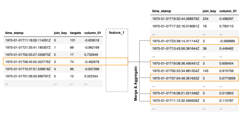
For example, such an aggregation could be the sum of all values in
column_01. We could also apply a subcondition, like taking only
values into account that fall into a certain time range with respect to
the entry in the population table. In SQL code such a feature would look
like this:
SELECT COUNT( * )
FROM POPULATION t1
LEFT JOIN PERIPHERAL t2
ON t1.join_key = t2.join_key
WHERE (
   ( t1.time_stamp - t2.time_stamp <= TIME_WINDOW )
) AND t2.time_stamp <= t1.time_stamp
GROUP BY t1.join_key,
     t1.time_stamp;
Unfortunately, neither the right aggregation nor the right subconditions
are clear a priori. The feature that allows us to predict the target
best could very well be e.g. the average of all values in column_01
that fall below a certain threshold, or something completely different.
If you were to tackle this problem with classical machine learning
tools, you would have to write many SQL features by hand and find the
best ones in a trial-and-error-like fashion. At best, you could apply
some domain knowledge that guides you towards the right direction. This
approach, however, bears two major disadvantages that prevent you from
finding the best-performing features.
You might not have sufficient domain knowledge.
You might not have sufficient resources for such a time-consuming, tedious, and error-prone process.
This is where getML comes in. It finds the correct features for you - automatically. You do not need to manually merge and aggregate tables in order to get started with a data science project. In addition, getML uses the derived features in a classical AutoML setting to easily make predictions with established and well-performing algorithms. This means getML provides an end-to-end solution starting from the relational data to a trained ML-model. How this is done via the getML Python API is demonstrated in the following.
Defining the data model
The next step is finding features in the data that allow an accurate
prediction of the target variable in the population table. This is
achieved using a MultirelModel. This model is responsible for the
entire process from feature engineering to predicting the target
variable based on the generated features. The MultirelModel requires
a predefined data model in order to efficiently represent the data in
memory. This is achieved via Placeholders. Placeholders are light
and abstract representations of DataFrames and their relations
amongst each other.
population_placeholder = population_table.to_placeholder()

peripheral_placeholder = peripheral_table.to_placeholder()

population_placeholder.join(peripheral_placeholder,
                            join_key="join_key",
                            time_stamp="time_stamp")
Now we can define the model. In addition to the Placeholders
representing the DataFrames you also have to provide a predictor.
Additionally, you can alter some hyperparameters like the number of
features you want to train or the list of aggregations to select from
when building features.
model = getml.models.MultirelModel(
    name='getting_started_model',
    population=population_placeholder,
    peripheral=[peripheral_placeholder],
    num_features=10,
    aggregation=[
        getml.models.aggregations.Count,
        getml.models.aggregations.Sum
    ],
    predictor=getml.predictors.LinearRegression(),
    seed=1706,
).send()
We have chosen a narrow search field in aggregation space by only
letting the model use Count and Sum. For the sake of
demonstration, we use a simple LinearRegression and construct only
10 different features. In real world projects you would construct at
least ten times this number and get results significantly better than
what we will achieve here.
Training a model
When fitting the model, we pass the handlers to the actual data residing
in the getML engine - the DataFrames.
model = model.fit(
    population_table=population_table,
    peripheral_tables=[peripheral_table]
)
Loaded data. Features are now being trained...
Trained model.
Time taken: 0h:0m:0.144649
That’s it. The Multirel feature engineering routines as well as the
LinearRegression contained in the MultirelModel are now trained
on our test data set.
Scoring the model
Let’s generate another population table as validation data set in order to see how well the trained model performs on new data. For numerical predictions this results in three different scores: mean absolute error (MAE), root mean squared error (RMSE), and the square correlation coefficient (rsquared).
population_table_score, peripheral_table_score = getml.datasets.make_numerical(
    n_rows_population=200,
    n_rows_peripheral=8000,
    random_state=1710
)

scores = model.score(
    population_table=population_table_score,
    peripheral_tables=[peripheral_table_score]
)
print("Mean absolute error: {:.3f}".format(scores['mae'][0]))
Mean absolute error: 0.005
Our model is able to predict the target variable in the newly generated data set very accurately.
Making predictions
You can also make predictions using the model you have just trained
population_table_predict, peripheral_table_predict = getml.datasets.make_numerical(
    n_rows_population=200,
    n_rows_peripheral=8000,
    random_state=1711
)


yhat = model.predict(
    population_table=population_table_predict,
    peripheral_tables=[peripheral_table_predict]
)
print(yhat[:10])
[[ 5.00268213]
 [14.00858787]
 [24.00367308]
 [ 1.00441267]
 [27.00394183]
 [20.00157795]
 [16.00315811]
 [ 4.00264301]
 [19.00271721]
 [25.00384922]]
Extracting features
Of course you can also transform a specific data set into the corresponding features in order to insert them into another machine learning algorithm.
features = model.transform(
    population_table=population_table_predict,
    peripheral_tables=[peripheral_table_predict]
)
print(features)
[[ 5.          0.99524429  5.         ...  0.26285526  0.26285526
  -0.31856832]
 [14.          3.80100605 14.         ...  3.15211846  3.15211846
   0.39465668]
 [24.          5.29167009 24.         ...  5.92441112  5.92441112
   0.12470039]
 ...
 [ 8.          2.00532951  8.         ...  0.94089783  0.94089783
  -0.74996369]
 [15.          1.90051102 15.         ...  2.11328521  2.11562428
  -0.72788024]
 [ 2.          0.6167304   2.         ...  0.05360352  0.05360352
  -0.35370042]]
If you want to see the SQL code for each feature, you can do so by
clicking on the feature in the monitor or calling the to_sql method
on the MultirelModel. The definition of feature_2 is
CREATE TABLE FEATURE_2 AS
SELECT COUNT( * ) AS feature_2,
       t1.join_key,
       t1.time_stamp
FROM (
     SELECT *,
            ROW_NUMBER() OVER ( ORDER BY join_key, time_stamp ASC ) AS rownum
     FROM POPULATION
) t1
LEFT JOIN PERIPHERAL t2
ON t1.join_key = t2.join_key
WHERE (
   ( t1.time_stamp - t2.time_stamp <= 0.499323 )
) AND t2.time_stamp <= t1.time_stamp
GROUP BY t1.rownum,
         t1.join_key,
         t1.time_stamp;
This very much resembles the ad hoc definition we tried in the
beginning. The correct aggregation to use on this data set is Count
with the subcondition that only entries within a time window of 0.5 are
considered. getML extracted this definition completely autonomously.
Next steps
This guide has shown you the very basics of getML. Starting with raw data you have completed a full project including feature engineering and linear regression using an automated end-to-end pipeline. The most tedious part of this process - finding the right aggregations and subconditions to construct a feature table from the relational data model - was also included in this pipeline.
But there’s more! Related articles show application of getML on real world data sets.
Also, don’t hesitate to contact us with your feedback.